Evolution of Distributed Training in Deep Neural Networks

We often view scientific progress as a series of sudden, transformative breakthroughs. In reality, progress is a continuous climb, with milestones marking new peaks. Deep learning’s evolution reflects this, built on years of iterative advancements in architectures like RNNs, CNNs, and attention mechanisms, culminating in the versatile transformer. Yet, the emergent behaviors of transformers, such as their remarkable generalization, only surface when models scale to billions of parameters. This scaling owes much to equally critical advancements in distributed training infrastructure, which enables efficient computation across hundreds or thousands of GPUs, unlocking the potential of massive neural networks. Join me as we explore the history and evolution of distributed training.

Why distributed training

The amount of GPU memory and FLOPS needed to train a model increases with the model parameter size and the input data. A napkin math approximation says the number of (compute) FLOPS needed is 6PD where;
P - Number of parameters, or model size
D - number of tokens that the model is trained on

For example, a 70B parameter model trained on 15T tokens would require a total flops of 6 * 70e9 * 15e12 = 6.3e24 FLOPS [1][2]. With a single H100 rated at 1979e12 FLOPS for fp16/be16 (with sparsity)[3] and a reasonable Model Flops Utilization (MFU) of 0.5, this would take 403 years! Clearly, we need to do things in parallel.

Similarly, the math for GPU memory is roughly = (Parameters + Gradients + Optimizer) + Activations
So with N parameters and using fp32 precision,
B: Batch size
T: Number of tokens per batch

Total Memory = (P (parameter) + P (gradient) + 2P (optimizer)) *4 + B * T * activation factor * 4
= 16P + B * T * k * 4

With P as 70B, Total memory = 1120G + activation cost (a few hundred MBs) which requires at least 14 H100 GPUs.

Without distributing the work across multiple GPUs, we will not get very far. Distributed training is splitting model training across multiple GPUs or machines to handle larger models and datasets faster. There are three broad and mutually non-exclusive ways to distribute the training.

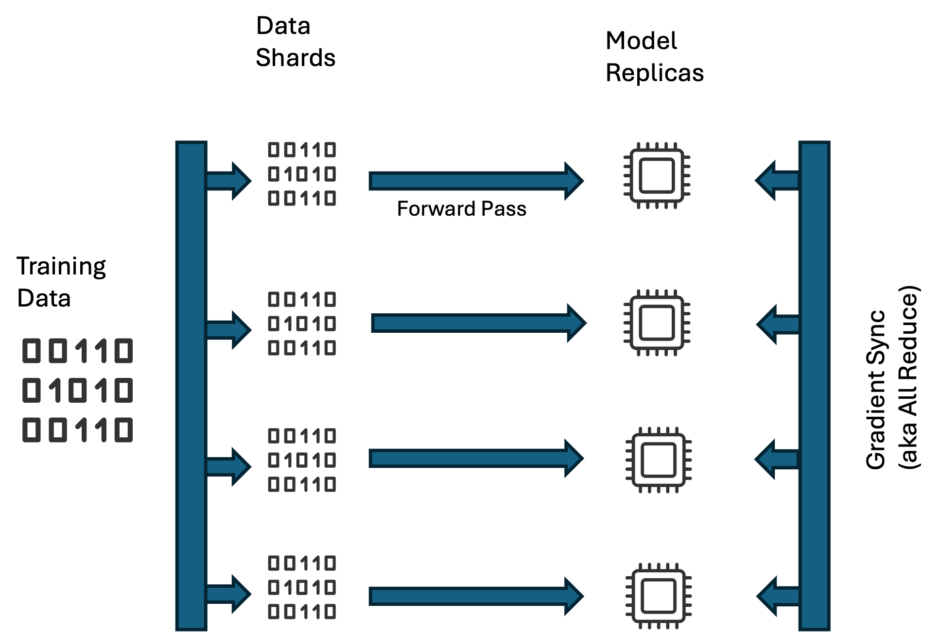
Data Parallelism

In this approach, imagine N replicas of the model running independently on different GPUs in a compute cluster, with the training data spilt into N shards. Each model instance is fed mini batches from its own data shard during the forward pass. The gradients w.r.t. the loss are computed independently on all the GPUs. These gradients are synced across all the GPUs using collective communication primitives like the NCCL All-reduce. Once all the GPUs have the same gradients, an optimizer update on each of the model replicas updates the parameters bringing them all in sync.

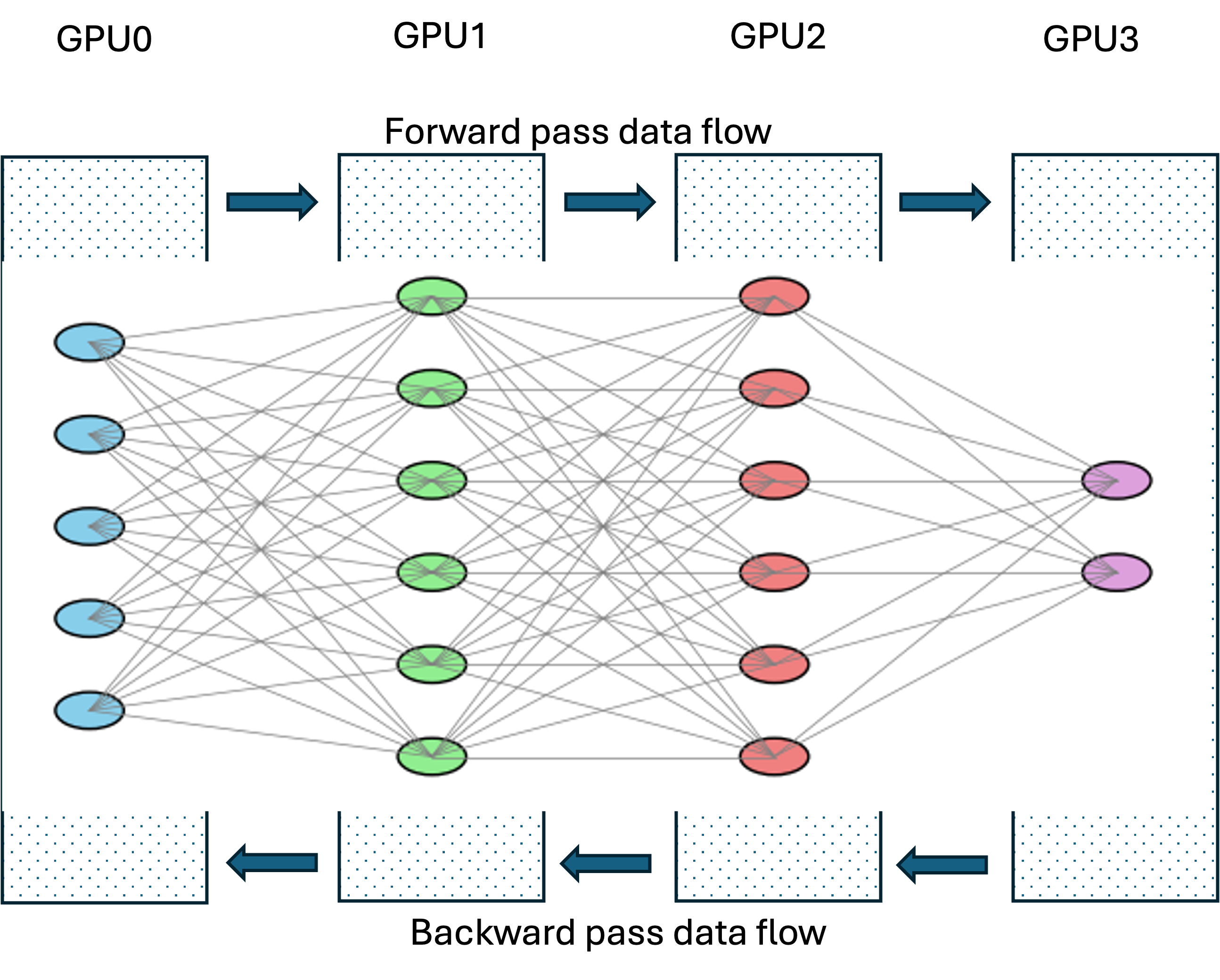
Model Parallelism

Recall how in our 70B parameter example, a single H100 (with 80GB of GPU memory) could not even hold a single copy of the model in memory. In such cases different layers of the model are distributed across GPUs. The model operates on small batch sizes. In the forward pass the activations from a layer are communicated to the next layer on another GPU using distributed computing primitive messages (e.g. NCCL Send). In the backward pass, gradients are computed layer by layer using saved activations, starting with the last layer, working its way back to the first. Since each stage holds a unique slice/layer of the model, there is no need to further sync the gradients. The optimizer step to adjust the parameters is done locally per stage/layer. This approach is called model parallelism.

Tensor Parallelism

In models with really large layers, it is quite possible that a single matrix multiplication might blow your GPU memory budget. To work around this problem, the work can be divided across multiple GPUs. For example, in a matmul of matrices A and B with dimensions M x N and N x O respectively, we can decompose matrix B into B1, B2, B3, B4, each of dimensions N x O/4, such that B1, B2, B3 and B4 carry shards of columns from B. Now a matmul of A with B1, B2, B3, B4, done separately, and joined together (via NCCL All-gather), will give the same result as a matmul of A and B. This is called tensor parallelism.



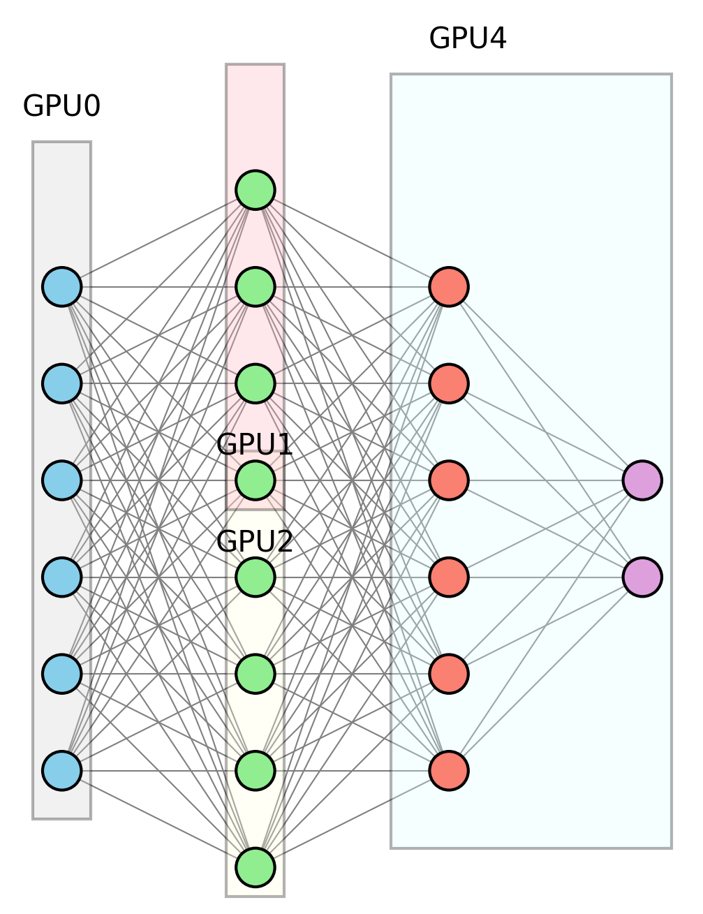
Above we can see the 2nd layer of the MLP split across GPU1 and GPU2. It is possible to use all three approaches simultaneously when training large language models.

Evolution of approaches to distributed training

As the scale of the models being trained increased, approaches to distributed training also changed on several axis. One axis was going from using CPUs to GPUs to CPU-clusters to finally GPU-clusters. Another axis was in the architecture used in gradient/state distribution. Yet another was in the topology, both logical and physical that the GPUs were arranged in to drive optimality.

DistBelief (2012)

In 2012, Jeff Dean et al.’s seminal paper, “Large Scale Distributed Deep Networks,” marked a turning point in deep learning by introducing scalable distributed training with the DistBelief framework[4]. GPUs were just beginning to transform neural network training. Researchers were concurrently recognizing that scaling model parameters and/or training data, could drastically improve model performance [5]. Existing infrastructure and I suspect expertise at Google lent itself better to using distributed computing across CPUs, as against trying to build a cluster of GPUs.

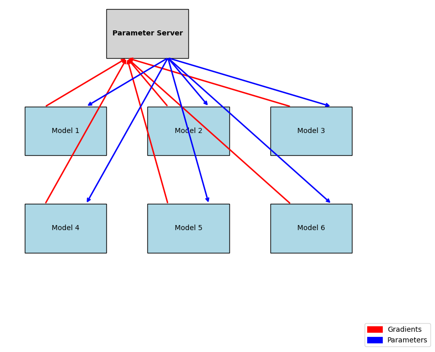
The DistBelief framework, pioneered scalable distributed training working well at scales of 32 machines, each with 16 CPU cores, for a total of 512 cores. It combined data parallelism and model parallelism, splitting computation within each replica across cores. At its core, a set of distributed parameter servers store and update model parameters, with each server holding a subset of the parameters. Before each forward pass, model replicas fetch the latest parameters from the server, compute gradients locally, and send them to the parameter server. The parameter server aggregates gradients from the various model replicas and performs the optimizer step to update the model parameters.

This approach, termed Downpour SGD, revealed a key insight: strict synchronization across replicas was unnecessary, as asynchronous updates still yielded robust performance. This meant at any given point, model replicas could be operating using different sets of parameters to compute gradients, making the process noisy. Despite this, DistBelief worked. This insight was empirically driven rather than grounded in good theory. However, it was soon discovered that this approach only worked well for smaller models and as models grew larger, asynchronous updates resulted in instability and poor convergence. Almost all distributed training assumes synchronous operation today.

NCCL - NVIDIA Collective Communications Library (2015)

After early adoption of the DistBelief parameter server model, the state of the art evolved to synchronous, collective-based training where parameter servers were replaced with more scalable collective operations with better integration of GPUs/TPUs. Collective communication libraries implement communication operations involving multiple processes or devices acting together, collectively, to perform a data movement or synchronization pattern across a group. This term comes from MPI (Message Passing Interface) [6] used in high performance computing. NCCL from NVIDIA is one such library that is loosely based on MPI, optimized for NVIDIA GPUs and for deep learning.

It has support for operations like:

AllReduce

Sum or reduce tensors across GPUs. This is the workhorse for synchronous SGD. When using PyTorch distributed training (DDP) each GPUs gradients are added together using NCCL all-reduce during the backward pass.

Broadcast

Broadcast tensor from one ‘root’ GPU to all others. This is used for initial model synchronization (so that all replicas start with identical weights) and any time one node has new parameters to share.

Reduce/ReduceScatter

Reduce tensors to a root GPU. ReduceScatter splits the reduced results across GPUs. Often a reduce-scatter operation is used as the first step in all-reduce, leaving the shards of reduced results spread across GPUs. A subsequent all-gather operation completes the all-reduce operation. This approach is taken to be bandwidth optimal.

AllGather

Gather tensors from all GPUs. This operation concatenates data from all GPUs and is used in practice when each GPU holds a shard of a tensor, and we want to gather the full tensor on each GPU.

While there are other collective libraries like Gloo and OneCLL, NCCL is the standard owing to better integration with NVIDIA GPUs and excellent integration with leading machine learning frameworks like PyTorch and TensorFlow.

Horovod and Ring Topology (2017)

With increase in model sizes and increase in GPU cluster sizes, it became clear that inter-GPU communication was becoming the bottleneck resulting in significant underutilization of GPUs [7]. Focus turned to ideas for optimizing the amount of information exchanged in the network or across GPUs. Uber took forward an idea from Baidu, where Ring-AllReduce, a concept from MPI, was implemented in a TensorFlow fork. This was essentially based on a distributed computing paper, Bandwidth Optimal All-reduce Algorithms for Cluster of Workstations [8].

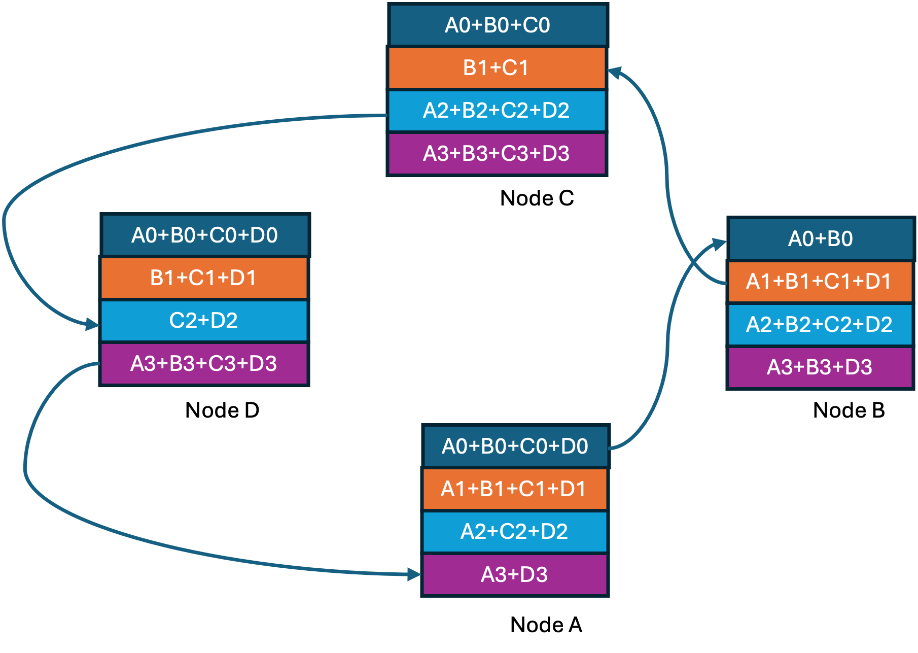
The idea here is to organize all the GPUs in a ring of N nodes, each communicating only with two of its peers/neighbors. Gradient data is sharded, with each node sending its shard to its neighbor on the right and receiving a shard from its neighbor on the left. The received gradients are added to its local data. In the next step this partially accumulated shard is sent to the peer on the right. At the end of N-1 steps, every node has N complete but different shards of the gradient data. This is followed by N-1 steps of each node distributing its completed shard to the right and receiving a completed shard from its left neighbor. At the end of this step all the peers have accumulated gradients, and the operation called ring-all-reduce is complete.

The below figure has four nodes/GPUs labelled A through D, with four gradient shards in each GPU numbered 0 through 3.

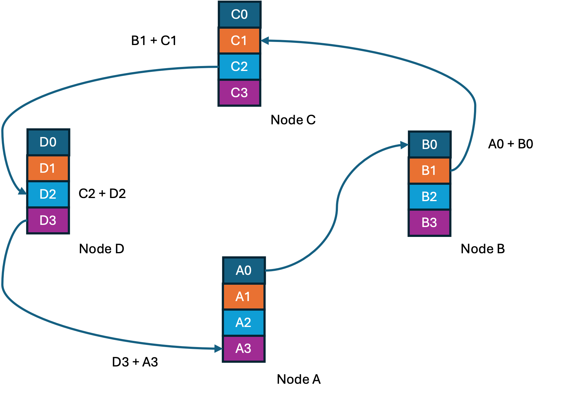
Step1 of 3 in Ring-Reduce

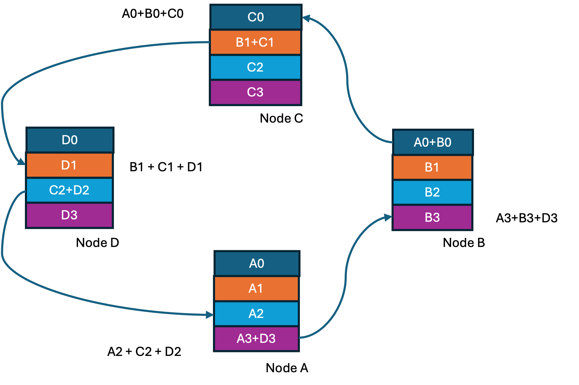
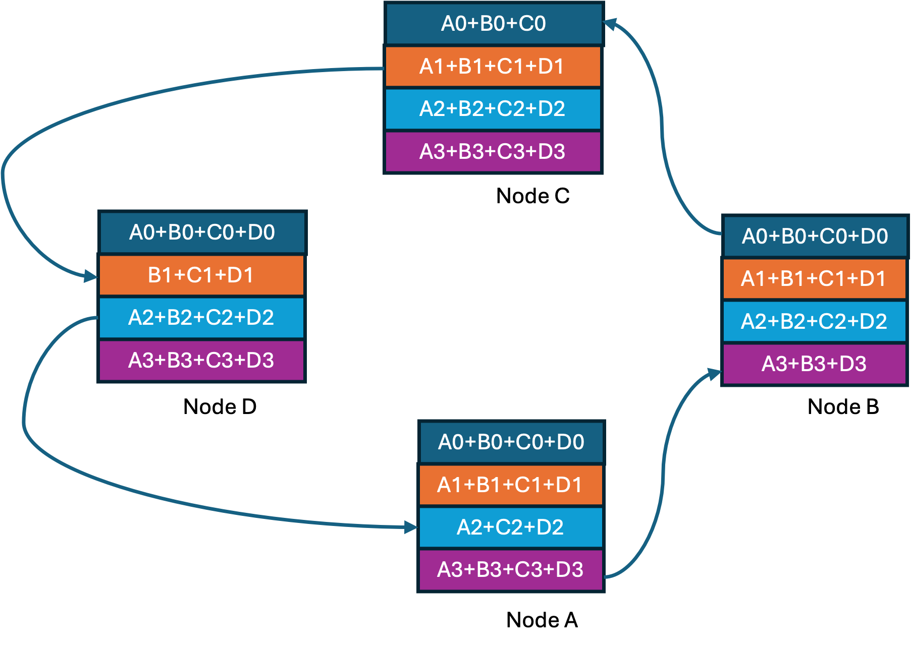
Step2 of 3 in Ring-Reduce

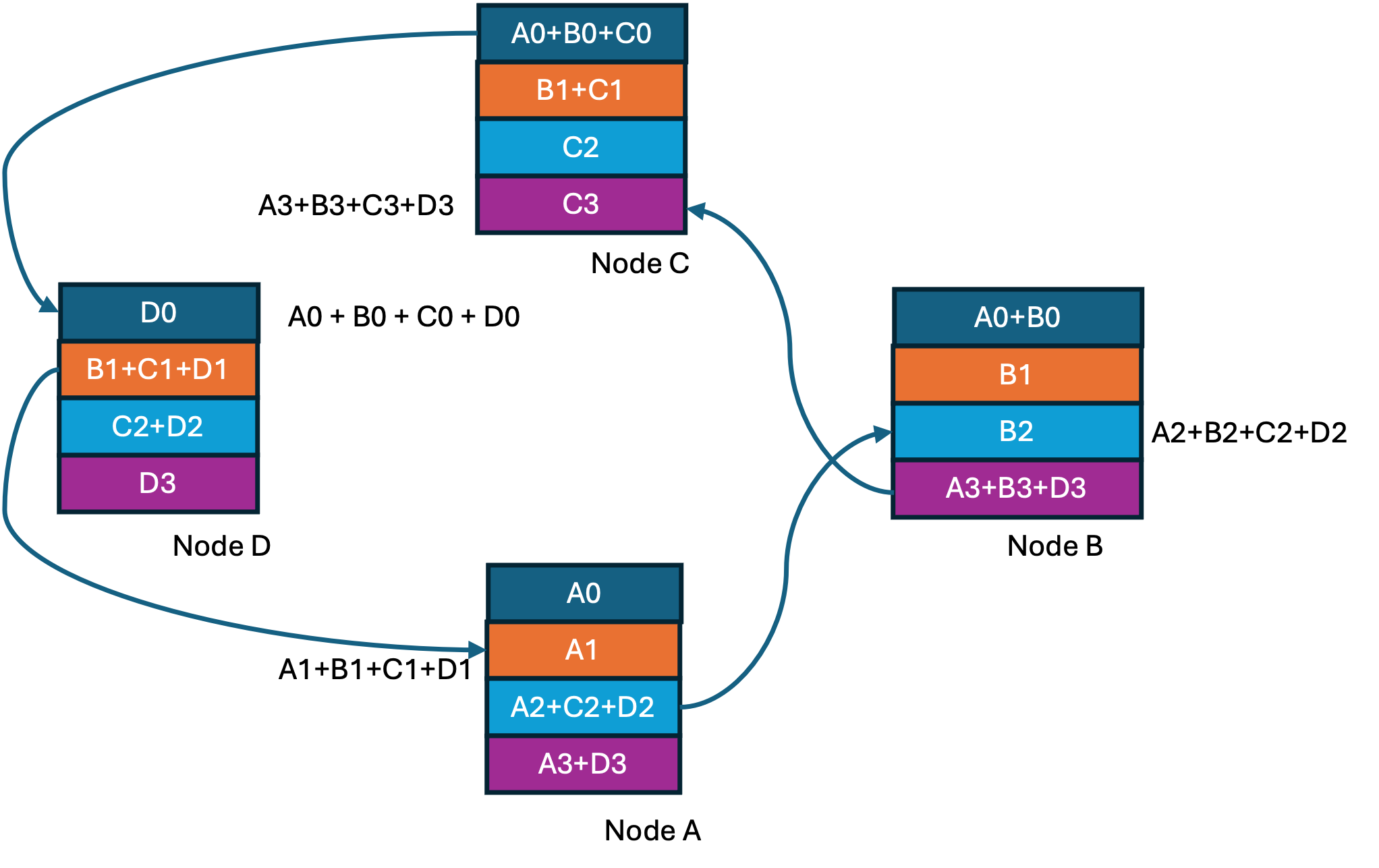
Step3 of 3 in Ring-Reduce

At the end of the ring-reduce we have every node having one completely accumulated gradient shard. Now we proceed to the ring-all-gather step shown below where at every step a completed shard is shared with the next node.

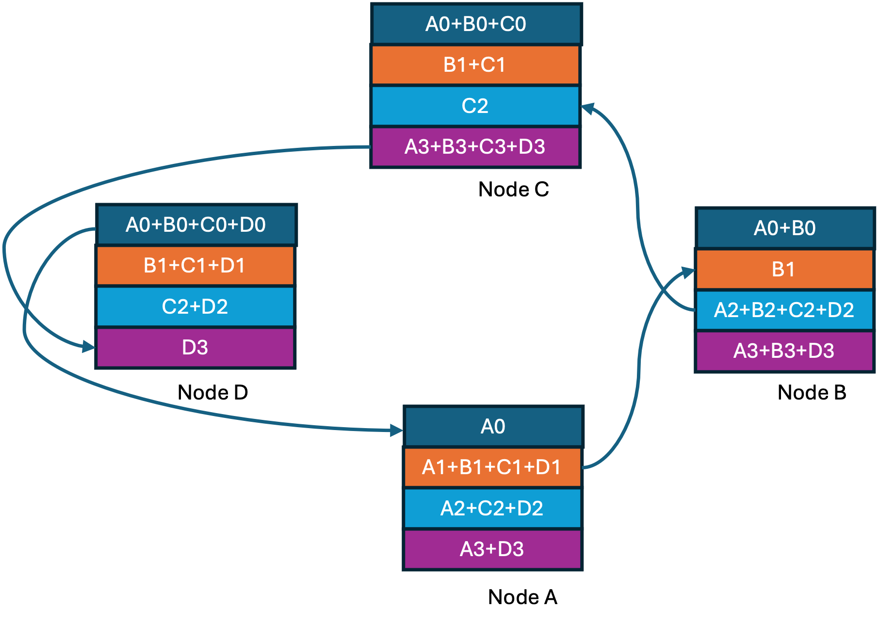
Step1 of 3 in Ring-all-gather

Step2 of 3 in Ring-all-gather

Step3 of 3 in Ring-all-gather

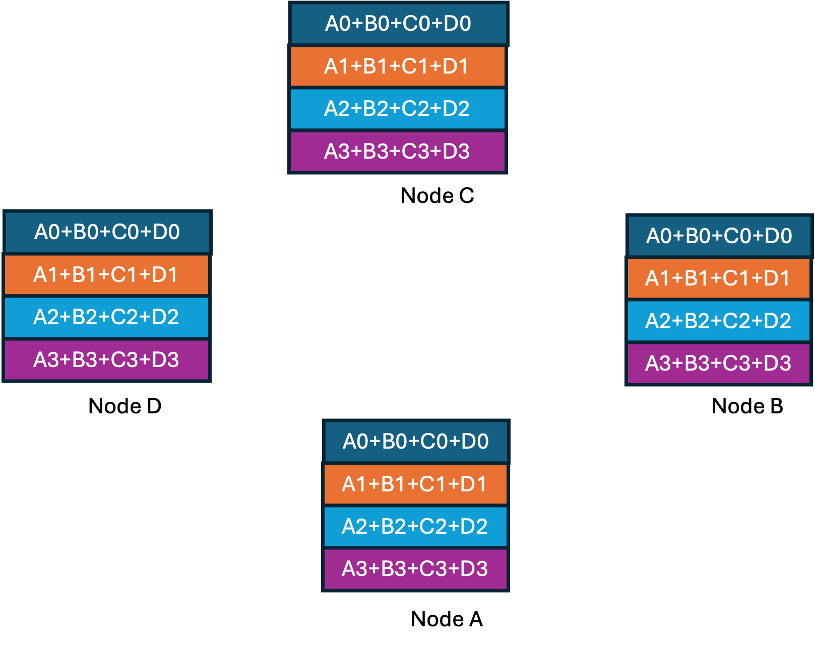
All-reduce completed

If you observe this approach, you will see that link bandwidth is optimally utilized with every GPU doing work in parallel. Uber released its implementation along with enhancements to simplify distributed training setup under a new framework named Horovod. This ultimately resulted in the ring-all-reduce approach already present in NCCL becoming more popular.

One problem remained with the ring topology, latency. As the number of GPUs grew into thousands, this became a problem. Optimizations and tweaks to the ring topology continued with Google in 2018 describing a 2D-ring approach where GPUs are connected in a Tourus-mesh with rings along the rows and columns of the mesh [12]. The data in each GPU is split along two dimensions, each dimension is further split into shards as you would in a typical ring. Both dimensions perform a ring-all-reduce simultaneously in the first step. Then the dimensions are swapped, and this process is repeated which results in an all-reduce over the entire data. This arrangement brings down the latency from \(O(N)\) to \(O(\sqrt{N})\).

Double Binary Tree Topology (2018)

Even with optimizations in ring, at large scale the latency introduced by rings becomes a problem. This was solved by introducing the double binary tree algorithm in NCCL [9]. This is again inspired from a distributed computing MPI idea [10].

At a very high level if the topology of the GPUs was arranged in a binary tree, we could perform an all-reduce operation in two stages. The first stage would be a reduction/summation starting at the leaf nodes that propagate gradients up the tree. This step can complete in log(N) time at which point the root of the tree has the reduced data. The second stage would be a broadcast down the tree from the root to the leaves. This does seem to solve the latency problem but introduces a link utilization problem. In the reduction phase, data is sent up the tree where two children feed data to a parent. So, parents have two sets of data coming in and one going out, causing imbalance and sub-optimal use of the links.

To solve this problem a second complimentary binary tree is created, were all the leaves of the first binary tree are nodes in the complimentary tree, and all the nodes are leaves in the complimentary tree. This means that every GPU has exactly two links coming in and going out. Now with the data sharded into two halves, you can imagine operating independently on these two halves over both these trees to perform the all-reduce operation while using all the links equally and optimally.

Hardware Advances in Distributed Training

Along with progress in algorithms and approaches to scale up distributed training, there have been significant advances on the hardware front focused on lossless connectivity between the GPUs.

RDMA over InfiniBand

The early days of scaling GPUs involved speeding up communication between GPUs on two different nodes/computers. Using traditional approaches like TCP/IP requires data in the GPU to come to the host memory over PCIe and then make its way out the NIC. With GPUDirect RDMA, released in 2011, NVIDIA and Mellanox demonstrated using RDMA over InfiniBand. This enabled direct data transfers between GPU memory and remote memory across nodes without involving the CPU or host memory.

NVLink

With designs having multiple GPUs on the same node, the NVLink interface was introduced. This provides a high-speed link between GPUs within the same node, avoiding the need to go through PCIe for GPU-to-GPU access. NVLink uses memory semantics allowing DMA and data sharing across GPUs. It started life as an intra node solution to speed up memory transfers across GPUs inside a node. However, recent designs have extended the NVLink domain outside the node using an NVLink switch. The idea is to support rack scale GPU pools, often needed for large model parallelism when dealing with models that do not fit in a single server.

UALink is a competing standards-based solution that aims to solve rack scale accelerator connectivity using memory semantics, with support from AMD and Intel among the GPU vendors. It will be interesting to see how this solution comes together and hits the market (end of 2025 or early 2026).

NeuronLink from Amazon is another high-speed interconnect using memory semantics designed to link GPUs and used in the AWS Neuron SDK stack as a chip-to-chip link within Trainium pods. Interestingly AWS today uses a 2D Torus mesh topology [13].

In-network Reduction (SHARP)

Another optimization in recent designs is the introduction of in-network reduction where instead of performing the reduction operation completely in a distributed manner, since the data passes through central points like an NVLink switch or an Infiniband switch, reduction operations could be performed in the network, and the results could be communicated to all the GPUs. This dramatically reduces the amount of data transferred. Today this is supported on NVSwitch (3rd Gen onwards) and some Infiniband switches.

RDMA over Ethernet (RoCE)

While some vendors are pushing Infiniband based solutions to cover training clusters spanning a data center, using Ethernet technologies is gaining traction. One key argument with Ethernet is that being standards based and more widely available, it reduces the total cost of ownership. While Infiniband is lossless, Ethernet with advances like Dynamic Load Balancing and enhancements through the Ultra Ethernet Consortium is closing the gap.

Scale Up Ethernet (SUE)(2025)

Since I first published this post, Broadcomm has announced Tomahawk Ultra that tries to tackle scale up of GPUs (or XPUs) using ethernet. The specification called SUE [14] seems to compete with NVLink for a piece of the scale up pie. It is also seems to compete with UALink so it is not quite clear what the strategy here will be long term. SUE does re-use a lot of ethernet though with a provision for using standard ethernet headers but also introduces what is coined as an AI Fabric Header (AFH). Here the source and destination mac addresses are compressed and source/destination XPU identifiers and other information makes its way in. The introduction of cell based flow control and link layer retransmissions brings loss less operation to this framework. Most importantly it seems to provide in-network reduction like NVIDIA does with SHARP. It is not clear though how end to end integration with collective libraries and the XPU NIC side will all work. From the announcement [15] it looks like this was a product designed for the HPC eco system which will find a lot of appeal in the AI training space. We have discussed the significant overlap in ideas in this space, so this is not entirely surprising. This sector is definitely fast moving.

Conclusion

Clearly, we are in a race to explore the limits of AI scaling laws. While initial results with DistBelief showed async training was possible, this fell apart quickly at scale. We are now in a synchronous training regime, with investments both in software and hardware aligned in support of this approach. All efforts are being expended to build larger and larger GPU clusters with hundreds of thousands of GPUs, all playing to the same metronome. On first principles as scale grows, problems with building a completely synchronous and lossless system are bound to get harder. There is a resurgence of research into asynchronous and partially asynchronous training for large-scale AI, including hierarchical async SGD, and federated approaches. These methods aim to overcome the inefficiencies and bottlenecks of synchronous training.

Perhaps a breakthrough in this space, the next big milestone, might reshape where things seem headed today?

References

[1] This excellent blog post by Dzmitry Bahdanau, The FLOPs Calculus of Language Model Training, explores the resources needed to train a model.
[2] Stanford CS336 Language Modeling from Scratch, Lec. 2: Pytorch, Resource Accounting.
[3] NVIDIA H100 Tensor Core GPU datasheet, page 2
[4] Large Scale Distributed Deep Networks, Jeff Dean et al., 2012 Distbelief
[5] ImageNet Classification with Deep Convolutional Neural Networks, Krizhevsky et al., AlexNet(2012)
[6] MPI: A Message Passing Interface Standard Version 5.0
[7] Horovod: Uber’s Open Source Distributed Deep Learning Framework
[8] Bandwidth Optimal All-reduce Algorithms for Clusters of Workstations
[9] Massively Scale Your Deep Learning Training with NCCL 2.4
[10] Two-tree algorithms for full bandwidth broadcast, reduction and scan (2009), Peter Sanders et al.
[11] NCCL: The Inter-GPU Communication Library Powering Multi-GPU AI
[12] Image Classification at Supercomputer Scale (2018), Chris Ying et al. 2D-Torus ring
[13] AWS Trn1 Architecture NeuronLink
[14] Scale Up Ethernet from Broadcomm SUE
[15] Tomahawk Ultra announcement TH Ultra