Reinforcement Learning - A TicTacToe Example
I’ll confess—the machine learning bug bit me later than most, and when it did, I was captivated by deep neural networks in the supervised learning setting. My early encounters focused on tasks like image classification, machine translation, and LLM challenges such as text generation. Most resources on transformer training highlighted the pretraining phase, which leverages self-supervised learning. It wasn’t until the DeepSeek R1 model’s release that I began to closely examine reinforcement learning (RL), a method that shines in sequential decision-making tasks like game-playing. Reflecting on it now, I’m surprised it took me so long to recognize RL’s value.
In this post, I dive into RL with a toy example: training a network to play tic-tac-toe using policy gradients, an approach where the model learns by optimizing action probabilities based on rewards. Let’s play against the resultant model below and explore how this was built.
What is running on your browser above is with the model weights converted from PyTorch into the ONNX (Open Neural Network Exchange) format and then run in javascript using onnxruntime-web. The code for this is available at https://github.com/pselect6/rl-toy-tic-tac-toe
What is Reinforcement Learning
Reinforcement learning (RL) is a branch of machine learning centered on training an agent to improve its performance by interacting with an environment and learning from experience. Unlike supervised learning, which relies on large labeled datasets to train a model to approximate a function, RL involves an agent that learns through trial and error, much like how humans iteratively adapt by exploring and receiving feedback. This approach powered breakthroughs like AlphaGo and AlphaZero, where DeepMind’s team developed networks that defeated the world’s best human Go player and outplayed Stockfish 8, the top chess engine at the time. At its core, RL involves an agent observing the environment’s state, taking an action that alters the state, and receiving a reward based on the action’s effectiveness—all aimed at maximizing the total reward over time. Get this process right, and your network can learn optimal behaviors for complex tasks.
Supervised Learning Primer
To better grasp RL, we start with a quick primer on supervised learning.
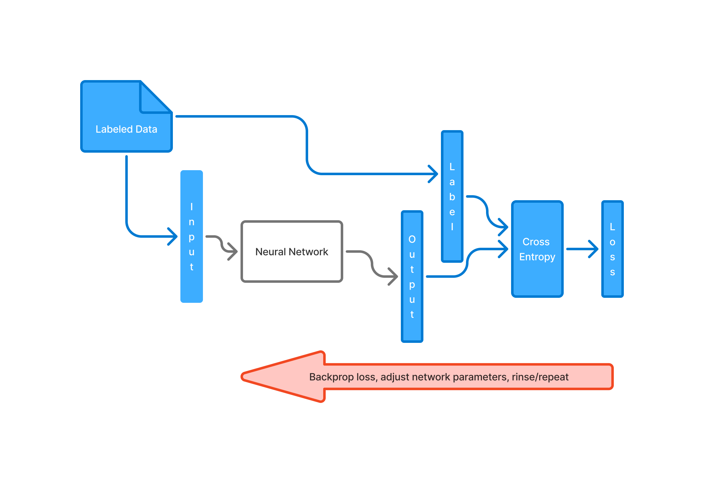
In supervised learning, you start with a labeled dataset containing inputs paired with their corresponding labels—the expected outputs. These inputs are fed into a neural network in batches, producing a batch of predictions. For a classification task, such as the one described, the network outputs a probability distribution over possible classes for each input. This predicted distribution, along with the true label, is passed through a cross-entropy loss function, which quantifies how far the network’s predictions deviate from the actual labels across the batch. (Cross-entropy, a fascinating concept rooted in information theory, measures the information content of an event, but that’s a topic for another day.) Using this loss, we backpropagate through the computation graph to compute the gradients of the loss with respect to the network’s parameters. These gradients guide us to update the parameters in the direction that reduces the loss, thereby enhancing the network’s performance over time.
Differentiability
All this is possible because the compute graph above is composed of differentiable operations. Every operation within the neural network all the way through to the computation of the loss is a differentiable function. The optimization step is rather simple, so is finding the parameter gradients using the calculus chain rule. What if the loss computation involved an evaluation of the network output through an opaque or non-differentiable reward function?
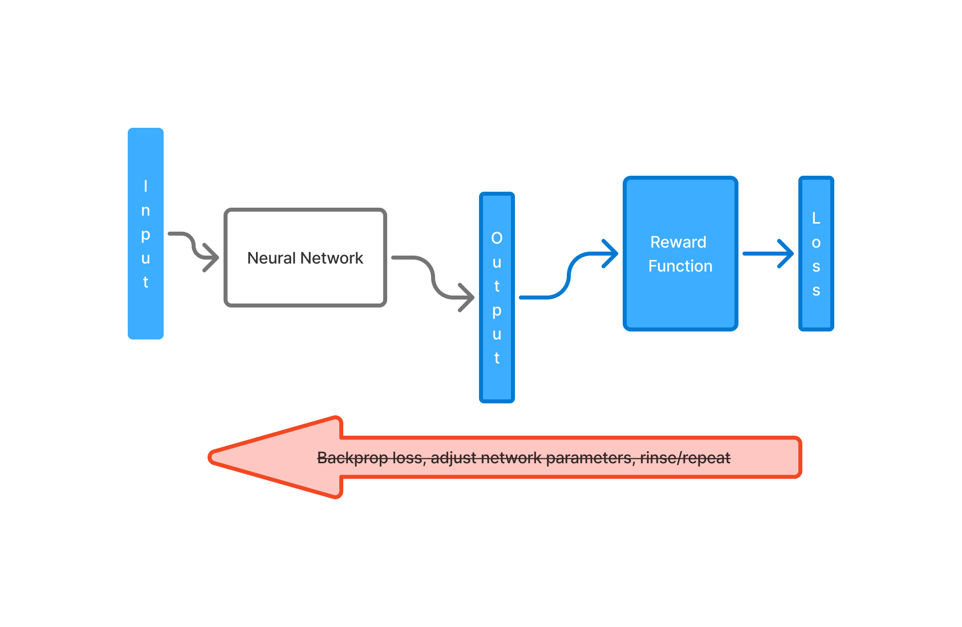
This non-differentiability or our inability to express the problem in terms of a simple differentiable objective function means that a lot of the tricks we learnt in supervised learning fail in this environment. As you can imagine, a large class of real work problems fall into this category. For example, in robotics, knowing if the action taken is good is not a differentiable operation. Playing a board game like chess where the number of legal positions is very large (over \(10^{43}\) attributed to Claude Shannon). Creating a labelled data set is impossible at this scale. Strictly speaking, beyond being non-differentiable there is also a problem of the reward being non-existant at each step. Often in a game setting, it is not immediately clear at every step if there is a reward associated with it.
Multiple Approaches to RL
There are several approaches to RL, each with its own advantages and tradeoffs.
The evolution based approach is a brute force gradient-free approach that does not exploit the structure of the problem. It simply treats the parameters \(\theta\) of the neural network as sampled from a Gaussian with mean \(\mu\) and variance \(\sigma\). The results of mutiple sets of parameter \(\theta\) samples are evaluated, a top performing (say 20) percentage of these are selected, a new \(\mu\) and \(\sigma\) are computed corresponding with these evolutionary winners and this process is repeated.
Markov Decision Process
There are Value-based methods using dynamic programming that define the RL problem as a Markov Decision Process (MDP). The Policy Gradient approach we focus on also uses the MDP framing. An MDP is formally defined by:
- s - set of states that describes the environment
- a - the action taken based on a policy \(\pi\)
- R(s,a,s’) - the reward for the action taken based on s, s’ (the new state) and a
- \(\boldsymbol{\gamma}\) - a discount factor for future rewards, prioritizing immediate rewards over distant ones
- H - the horizon or the maximum time steps we play for
- P - the probability P(s’|s,a) that defines the transition from s -> s’ given an action a.
This describes the dynamics of the environment, specifically how likely you will land in s’ given s and a. In a board game setting, this is deterministic, but in a robotics setting you can imagine why this is needed.
Imagine a game where an agent has a view of its environment through state ‘s’, decides on an action ‘a’ to be taken based on a policy \(\pi^{*}\). Each action taken results in a possible reward. There is an immediate reward and the possibility of future rewards for subsequent actions taken. Future rewards are less important than immediate rewards, hence these are attenuated by a discount factor \(\gamma\). The game is played upto a maximum number of steps, the horizon.
The goal of an MDP is to find an optimal policy \(\pi^{*}\) that maximizes the cumulative discounted reward.
\(\) \(\pi^{*} = \underset{\pi}{argmax}\:\mathbb{E}[\sum_{t=0}^{H}\gamma^{t}R(s_{t},a_{t},s_{t+1})|\pi]\)
Value Methods
The Q-learning approach uses dynamic programming to find the optimal Q value for a (s, a) using the bellman equation. The Q value is simply a value that represents the cumulative reward if from state ‘s’ the action ‘a’ is performed, followed the best possible action from the new state s’.
\(\) \(Q^{*}(s,a) = \underset{s'}{\sum}P(s'|s, a)(R(s,a,s') + \gamma\: \underset{a'}{max}Q^{*}(s',a'))\)
Iterate the below equation enough times to converge to the optimal Q value. In a given state, the action with the highest Q value gives the optimal policy \(\pi^{*}\).
\(\) \(Q^{*}_{k+1}(s,a) = \underset{s'}{\sum}P(s'|s,a)(R(s,a,s') + \gamma\: \underset{a'}{max}Q^{*}_{k}(s',a'))\)
We will be focussing on the Policy Gradient approach that uses the MDP framing and has parallels to supervised learning.
Policy Gradients
This is the branch of RL methods that directly tries to get to the optimal policy to be used. In the Q-value methods, we compute the value associated with a (state,action) pair and indirectly find the optimal policy as a side effect. In other words the action that corresponds to the highest Q-value becomes the recommended policy action.
The policy gradient idea is to directly model the policy as a neural network. The policy takes in the state and outputs a probability distribution over all possible actions. This means we now have a stocastic policy class that presents the actions in a probabilistic manner. This allows smoother tuning of the distribution over actions which is ideal for algorithms like SGD to work.
There is a bit of terminology and math that helps build some intuition for the method. This is useful to understand and not very complicated if you have the time. Alternatively, the pytorch code might be an easier read so feel free to skip the math. Most of the math and notation is pretty standard and the material is all from the Deep RL Bootcamp 2017. The lectures on Policy Gradients are definitely worth a watch. As usual Karpathy’s blog on Policy Gradients is very accessible.
Trajectory
Let \(\tau\) denote a state-action sequence \(s_{0},u_{0},...,s_{H},u_{H}\) where \(\tau\) represents the trajectory of state action pairs. Each trajectory represents the state changes and moves from an episode of game play. Remember how in a game setting, every move might not immediately offer a reward so it is easier to imagine rewards associated with a trajectory or a complete episode of a game.
\(R(\tau) = \sum_{t=0}^{H-1} R(s_{t},u_{t})\) ; the cumulative reward for a trajectory \(\tau\)
Our goal (ignoring the discounting factor \(\gamma\)) is to maximize
\(\) \(U(\theta) = \mathbb{E}[\sum_{t=0}^{H} R(s_{t}, u_{t});\pi_{\theta}] = \sum_{\tau} P(\tau;\theta)R(\tau)\:\:\:\:\:\:\:\) # definition of expectation
Expectation is simply the probability weighted average of a value.
Here \(P(\tau;\theta)\) is the probability output of our neural network.
\(\) \(\underset{\theta}{max}\:U(\theta) = \underset{\theta}{max}\sum_{\tau}P(\tau;\theta)R(\tau)\)
To maximize \(U(\theta)\) we find the gradient of our objective function \(U(\theta)\) so that we can move in this direction.
\(\) \(\Delta_{\theta}U(\theta) = \Delta_{\theta}\sum_{\tau}P(\tau;\theta)R(\tau)\)
\(\) \(\Delta_{\theta}U(\theta) = \sum_{\tau}\Delta_{\theta} P(\tau;\theta)R(\tau)\:\:\:\:\:\:\:\:\:\:\:\:\) # gradient of sum is same as sum of gradients
\(\) \(\Delta_{\theta}U(\theta) = \sum_{\tau}\frac{P(\tau;\theta)}{P(\tau;\theta)}\Delta_{\theta} P(\tau;\theta)R(\tau)\)
\(\) \(\Delta_{\theta}U(\theta) = \sum_{\tau}P(\tau;\theta)\frac{\Delta_{\theta} P(\tau;\theta)}{P(\tau;\theta)}R(\tau)\:\:\:\:\:\:\:\:\:\:\) # just some clever rearrangement of the terms
\(\) \(\Delta_{\theta}U(\theta) = \sum_{\tau}P(\tau;\theta)\Delta_{\theta} log P(\tau;\theta)R(\tau)\:\:\:\:\:\:\:\:\:\:\) # chain rule \(\delta(log(x)) = \frac{\delta(x)}{x}\)
\(\) \(\Delta_{\theta}U(\theta) = \mathbb{E}[\Delta_{\theta} log P(\tau;\theta)R(\tau)]\:\:\:\:\:\:\:\:\:\:\:\:\:\:\:\:\:\) # definition of expectation
Once we have an expectation we can approximate it by taking sample based estimate of the expectation. After all an expectation is simply the weighted average value based on the probability distribution. This is a quantity that can be approximated using Monte Carlo methods (using random sampling).
\(\) \(\Delta_{\theta}U(\theta) \sim \hat{g} = \frac{1}{m}\sum_{i=1}^{m}\Delta_{\theta}log P(\tau^{(i)};\theta)R(\tau^{(i)})\)
Key Result - Optimization Possible on Opaque Reward Functions
This is impressive in that without knowing anything about the nature of the reward function, we are able to optimize the policy network to maximize the reward. So we seem to have a way out of needing our reward function to be differentiable. Now lets focus on how this can be used in practice since we deal in small time steps, not at the granularity of trajectories.
Decomposing the trajectory into individual state and actions
\(\) \(\Delta_{\theta}\:log P(\tau^{(i)};\theta) = \Delta_{\theta} log [\prod_{t=0}^{H-1}P(s^{(i)}_{t+1}|s^{(i)}_{t}, u^{(i)}_{t}) . \pi_{\theta}(u^{(i)}_{t}|s^{(i)}_{t})]\)
\(\) \(\Delta_{\theta}\:log P(\tau^{(i)};\theta) = \Delta_{\theta} [\sum_{t=0}^{H-1} log P(s^{(i)}_{t+1}|s^{(i)}_{t}, u^{(i)}_{t}) + \sum_{t=0}^{H-1} log\: \pi_{\theta}(u^{(i)}_{t}|s^{(i)}_{t})]\)
Above becuase log of product of terms is the same as sum of log of the terms
\(\) \(\Delta_{\theta}\:log P(\tau^{(i)};\theta) = \Delta_{\theta} [\sum_{t=0}^{H-1} log\: \pi_{\theta}(u^{(i)}_{t}|s^{(i)}_{t})]\)
Above because the system dynamics or the probability of a next state given an initial state and action does not depend on \(\theta\) hence is zero
\(\) \(\Delta_{\theta}\:log P(\tau^{(i)};\theta) = \sum_{t=0}^{H-1} \Delta_{\theta}\: log\: \pi_{\theta}(u^{(i)}_{t}|s^{(i)}_{t})\)
\(\) \(\Delta_{\theta}U(\theta) \sim \hat{g} = \frac{1}{m}\sum_{i=1}^{m}\sum_{t=0}^{H-1} \Delta_{\theta}\: log\: \pi_{\theta}(u^{(i)}_{t}|s^{(i)}_{t})R(\tau^{(i)})\)
So what this informs us is that we can simply sum up the log probability of the individual actions that are part of the trajectory, compute its gradient and this is the same as gradient of the log probability of the trajectory. So in the episodic context, the individual actions can be sampled and its log probability summed up, then the gradient of this value will be the same as the gradient of the log probability of the trajectory. Once this value is available, this can be scaled by the reward associated with the outcome for the trajectory and finally the average of this over multiple episodes will form a batch over which you can backpropagate. This approach will move the parameters of the network in the direction that will increase the reward.
Notice how the system dynamics (probability of the action succeeding to transition into a state) does not figure anywhere in the optimization logic.
Reward Baselining
Now a major problem with trying to optimize the network in a direction of improving rewards is that the current formula will incentivize all the trajectories that result in a positive reward. However what we really want is to incentivize better than average performance and disincentivize weaker than average performance. To this end we subtract a quantity ‘b’, known as the average reward or baseline.
\(\) \(\Delta_{\theta}U(\theta) \sim \hat{g} = \frac{1}{m}\sum_{i=1}^{m}(\sum_{t=0}^{H-1} \Delta_{\theta}\: log\: \pi_{\theta}(u^{(i)}_{t}|s^{(i)}_{t}))\:[R(\tau^{(i)}) - b]\)
\(\) \(\Delta_{\theta}U(\theta) \sim \hat{g} = \frac{1}{m}\sum_{i=1}^{m}(\sum_{t=0}^{H-1} \Delta_{\theta}\: log\: \pi_{\theta}(u^{(i)}_{t}|s^{(i)}_{t}))\:[\sum_{t=0}^{H-1} R(s^{i}_{t},u^{i}_{t}) - b]\)
The baseline computation has a lot of options, the simplest being computing the average reward from a batch of rollouts and using this as the baseline.
Rewards To Go
The actions \(u_{t}\) should interact with all future rewards including the current time step because the current action influences future actions as well. However, the current action should not interact with previous rewards. Fixing this reduces the variance in the computation. We will see with our tic-tac-toe example how the network trains better when rewards-to-go is enabled.
\(\) \(\Delta_{\theta}U(\theta) \sim \hat{g} = \frac{1}{m}\sum_{i=1}^{m}(\sum_{t=0}^{H-1} \Delta_{\theta}\: log\: \pi_{\theta}(u^{(i)}_{t}|s^{(i)}_{t})\:\:[\sum_{k=0}^{t-1} R(s^{i}_{t},u^{i}_{t}) + \sum_{k=t}^{H-1} R(s^{i}_{k},u^{i}_{k}) - b])\)
Eliminating the usage of older rewards for future time steps, we get
\(\) \(\Delta_{\theta}U(\theta) \sim \hat{g} = \frac{1}{m}\sum_{i=1}^{m}\sum_{t=0}^{H-1} \Delta_{\theta}\: log\: \pi_{\theta}(u^{(i)}_{t}|s^{(i)}_{t})[\sum_{k=t}^{H-1} R(s^{i}_{k},u^{i}_{k}) - b]\)
Actor-Critic Methods
The baseline ‘b’ is not really a constant and ideally should be a function of the state. So this can be further refined as
\(\) \(\Delta_{\theta}U(\theta) \sim \hat{g} = \frac{1}{m}\sum_{i=1}^{m}\sum_{t=0}^{H-1} \Delta_{\theta}\: log\: \pi_{\theta}(u^{(i)}_{t}|s^{(i)}_{t})[\sum_{k=t}^{H-1} R(s^{i}_{k},u^{i}_{k}) - b(s_{t})]\)
Thinking more carefully about this, the baseline reward at each state is really the Value function at that state, \(V(s_{t})\) as this is the cumulative reward associated with the state.
Another neural network can be used to approximate the value function. When used in this mode, the policy gradient method is also called the Actor-Critic method. The actor being the policy network and the critic being the value function approximator.
Training a Model to Play TicTacToe
With the theory out of the way, we attempt to use this theory on a simple problem of teaching a model to play tic-tac-toe using RL. The idea is to put to test the various concepts RL to this toy example and gain some intuition for the training process.
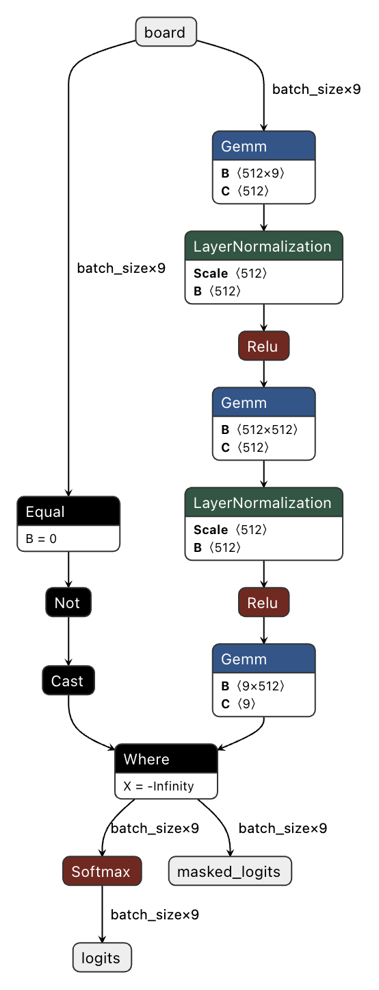
The model being trained is a simple MLP, taking in an input of 9 tensors, representing the 9 positions of a tic-tac-toe board. The first layer is a simple 9x512 Linear layer (General Matrix Multiply). There is a single hidden Linear layer of 512x512 followed by the output layer of 512x9 that outputs the logits over 9 possible moves followed by a SoftMaxlayer and masking to disable invalid moves. I use Relu as the non linearity and Layer Normalization before the Relu to keep the weights in shape. This is way too big for the size of the problem, but my focus was on the training process and having an oversized model does make the training easier.
Training Stages
The training loop uses a batch size of 50 (by default), picking a random first mover for a new game, goes on for 500000 games, summarizing the win/loss/draw statistics every 5000 games. During training we sample from the output probability distribution using torch.multinomial() to encourage exploration as against using an argmax (which would pick the highest probability). The reward model sets WIN_REWARD=1.0, LOSS_REWARD=-2.0, DRAW_REWARD=-0.6. So losses are penalized quite heavily, so are draws but to a lesser extent. The training results below are with entropy regularization and rewards-to-go enabled.
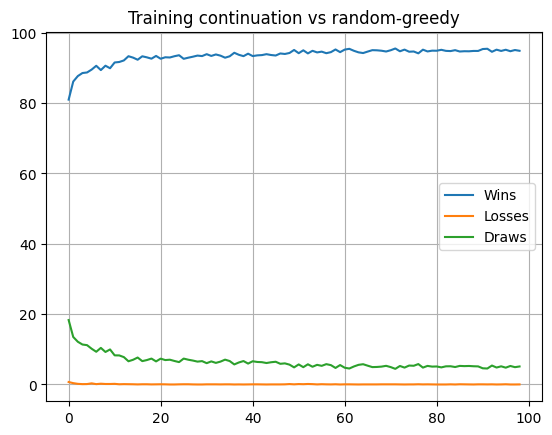
Start training from scratch against a ‘random-greedy’ opponent who makes random moves, except when there is an opportunity to win in one or prevent a loss.
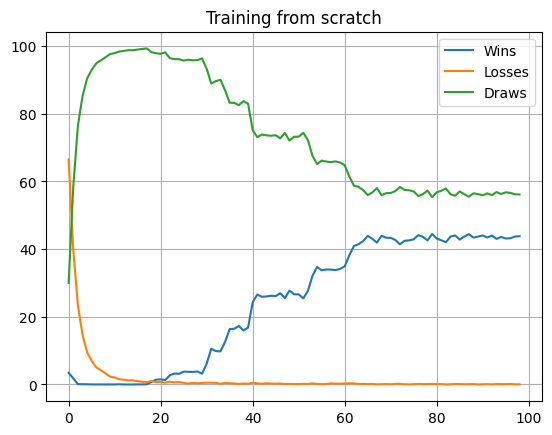
As you can see above, a model starts off with 70% losses, 3% wins, and improves. It is interesting to see how the losses drop first as the draws increase as the model penalizes losing quite heavily. During this window the wins actually decline. In general when training deep networks patience is key, but this is more so when doing RL. The input data your model encounters is not independent and identically distributed (IID) like in supervised learning. The training process takes your model through different environment states, so it is not uncommon for performance to drop before it improves so waiting it out when the performance dips is key.
Continue training against this opponent to get the loss percentage down to near zero.
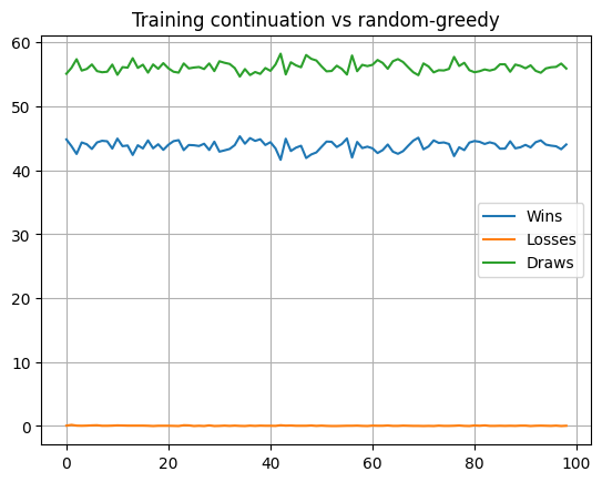
Sort out any kinks in the policy by playing against a true ‘random’ opponent.
Here you can see how even after multiple rounds of training against a ‘random-greedy’ opponent, this model still started off with a few losses against an inferior ‘random’ opponent. It also needed to learn how to capitalize on opponent mistakes better with the win% improving before it stabilized. The slight jitter in losses can be explained by our using torch.multinomial() when picking an action which means we do explore and make mistakes while learning.
Key Takeaways
Some of my subjective takeaways from this excercise.
-
Reward model matters the most
Most of my bugs were in the formation of the reward model. This is after all the objective function that the model is trying to optimize for so any subtle bugs here can be fatal. Even for a simple game like tic-tac-toe, I had a fair share of kinks to work out. For example, a straight reward of 1 for wins and -1 for losses did not work well given this game has a perfect solution where no loss is possible and wins against a good opponent should be impossible. So the learning aspect has to in some sense factor in the opponent you are playing against. I also settled on a negative reward for draws to encourage the model to find a win. A positive reward for draws can result in the model reward hacking its way into always settling for a draw when a win is possible. -
Rewards-to-go is Essential
The idea with rewards-to-go is to have the current action be incentivized by all future rewards. This knob is enabled by default and for a good reason. Without this, the model takes a lot longer to converge as the objective function will have a lot higher variance. -
Entropy regularization works
It is very clear that convergence improves with entropy regularization. The idea of rewarding the model for being less confident in its output or less peaked around a single action is key to exploration. The entropy here is simply the average of the log probability over all the actions predicted from the model and adding this to the objective encourages a more diverse set of actions, better exploration. -
Please set a seed for random
During training, be sure to set a fixed seed for your PRNG. Without this you will suffer, wondering why the performance dropped with code rearrangement, or celebrate premature success with hyperparameter changes that are unreproducible. Ideally you need to run your evaluations against multiple different seeds. Setting a seed gives you reproducible results without which you can’t even tell which way is up. -
Training logs are important
Nothing works the first time and the process is going to be iterative with multiple tweaks to the reward model, hyper-parameters, learning settings. Recognize the need to log all your tunables along with your training results, so that you can look at this later and not lose your head trying to figure out what changed. This does not need to be very complex, just need to capture everything you might ever tune. -
Inspect your values
Inspect the values coming out of your model, the log probabilities and entropy. Build an intuition for what happens to these values as training progresses. As the model becomes more confident in its output, the probability approaches 1, the log value approaches zero and hence the feedback when multiplied by the reward diminishes. During the early phase, there is higher entropy which drives a higher loss value, implying larger steps. For a while I thought I needed more exploration than what torch.multinomial() would allow, tried using an epsilon greedy approach of sampling a random action. This resulting in my picking some really low probability actions, which have high negative log probabilities. This ended up with high gradients and my model output generating NaNs. So inspect your values, understand the dynamics at play and build an intution for how all this is working at the numerical level.
Conclusion
Although tic-tac-toe, the toy example I chose, doesn’t demand a complex neural network and could be tackled with a simpler algorithm, it serves as an ideal case to demonstrate RL training in action. Several topics still warrant deeper investigation: Why didn’t reward baselining improve performance? Could a true Actor-Critic model address the baselining issue? Might tabular Q-learning offer a more straightforward solution? Theory and intuition can only take you so far—there’s no substitute for hands-on experimentation, which I plan to dive into soon. Thanks for reading, and I’d love to hear your thoughts.