Why don't neural nets get stuck?
Why is it possible to optimize a neural network and how does this optimization really work? The general idea with neural network training at least in the supervised learning setting, is to define an objective function that when optimized, sculpts the network parameters into producing accurate predictions over the training data. The network starts off with its parameters initialized randomly, or using some other heuristic. The objective function (or loss function) measures how far the networks predictions are from the true labels in the training data. We progressively tweak the network to reduce the loss. How can we be sure that this loss function can be navigated to find the optimal parameters of the neural network?
Navigating the Loss Landscape
The loss function \(L_{\theta}(X,Y)\) is dependent on the network parameters \(\theta\) and the input X and corresponding true label Y.
The general idea in optimization is to have a (hopefully) convex loss function over which algorithms like stochastic gradient descent (SGD) can run and find a good minima. The idea is to adjust the network parameters \(\theta\) such that the loss is minimized. This is done by computing the gradients of the loss with respect to the network parameters \(\theta\). Now recall that \(\theta\) is actually a vector, so we are really computing partial derivatives. Once the gradients are known the algorithm descends the loss surface by gradually moving the parameters in the opposite direction of the gradient.
The natural question that should come up is, would the optimization algorithm get stuck in a local minimum, or a point in the loss surface that has an increasing loss in all directions, stuck in a ditch so to speak. This belief used to dominate machine learning and there was an obsession with making sure your loss function is convex.
Convexity
Mathematically, a function \(f:R^{n} \rightarrow R\) is convex if, for any two points \(x_{1}\) and \(x_{2}\) in its domain and for any \(\lambda \in [0,1]\), the following inequality holds:
\(f(\lambda x_{1} + (1-\lambda)x_{2}) \le \lambda f(x_{1}) + (1-\lambda) f(x_{2})\).
Simply put,
\(\lambda x_{1} + (1-\lambda)x_{2}\) is every point between \(x_{1}\) and \(x_{2}\) as you decrease \(\lambda\) and
\(\lambda f(x_{1}) + (1-\lambda) f(x_{2})\) is every point between the function values at \(x_{1}\) and \(x_{2}\), \(f(x_{1})\) and \(f(x_{2})\).
So convexity requires that the function value be below any chord drawn over the function. It also means that any local minimum of a convex function is also a global minimum.
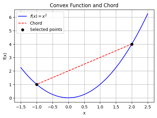
This intuitively makes sense, to avoid getting stuck in a smaller hole in the loss surface like in the example below.
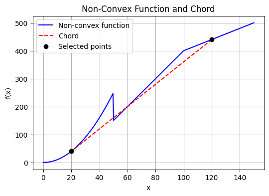
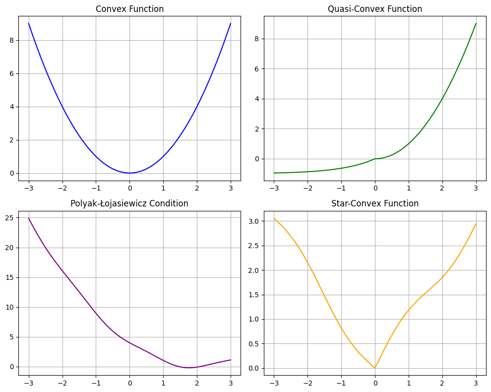
However, this is overtly restrictive as clearly all the below functions, not all of them convex, present optimizable surfaces. So convexity is a sufficient but not necessary condition.
In reality most loss functions in the deep learning setting are not convex. The network with its multiple layers of non-linearities (like RELU, GELU, Sigmoids etc.) are highly likely to have a non convex loss function. So what does this mean for gradient descent down the loss function? Should we not get stuck in a local ditch more often?
High Dimensional Spaces to the Rescue
With deep learning, the number of parameters in a neural network exploded with most networks sporting millions of parameters. For example the VGG16 image classification network has 138M parameters, the BERT models range from 4.4 million to 340 million parameters. The GPT and LLM class of models take this even further with hundreds of billions of parameters. This means our loss function \(L_{\theta}\) is trying to navigate a highly dimensional space with millions of parameters. With this a new realization emerged: the local minima problem might not be as bad as feared.
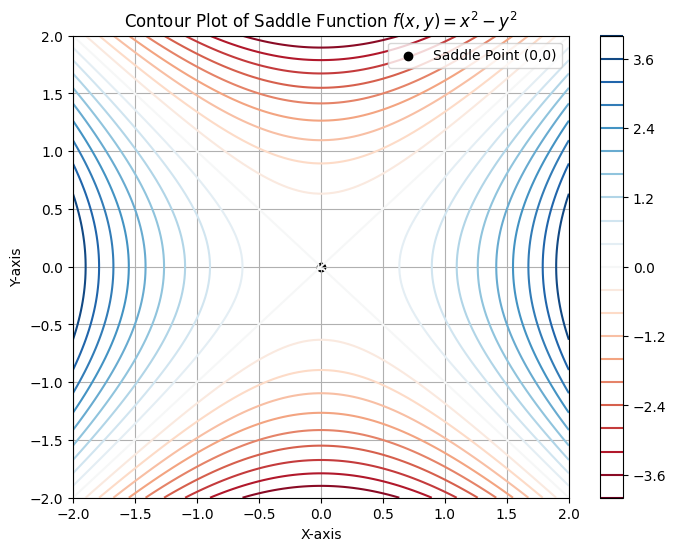
The geometry of the loss landscape in high dimensions is very different when compared to low dimensions (e.g. 2D, 3D) where the loss surface can have definite peaks, valleys and plateaus with local minima that can trap you. A local minima requires the surface to curve upwards in all directions around the point, something that is intuitively harder when there are higher numbers of dimesions and hence larger number of directions involved. Mathematically (and this is not really that important to understand), this requires the Hessian matrix to be positive definite, which means all its eigen values should be positive. This becomes highly unlikley as the dimensions increase. If the Hessian matrix has some positive and some negative eigen values, this means the surface is a saddle point, not a local minima. So the math here is effectively indicating that in highly dimensional spaces, it is more likely that the loss surface encounters a saddle point than it will encounter a local minima. Now saddle points always have an off ramp and while it can have flat gradients along some directions, there always exists a direction that results in a lower loss. SGD with enough entropy due to the stochastic nature of selecting mini batches of the input should find the off ramp.
Empirical results training deep neural networks also show that the fear of local minima seem overblown. The simple SGD method seems to work quite well. Often when discussing the need for SGD, one assumes that the need for running the loss computation in mini batches of the data comes from memory and compute limitations. While partially true, the stochastic selection of the input data has a regularization effect that introduces sufficient noise in the loss computation that can help with getting over smaller undulations in the loss surface.
Learning in High Dimensional Spaces
When the number of parameters of a network is increased, empirically we observe that the network is easier to train. This could be interpreted as a shift in the nature of the loss landscape that allows SGD to work. As networks grow larger, the loss surface tends to become smoother and more convex-like. Is there an optimal parameter size and a principled way to size this?
One way of analyzing this is the redundancy added when parameters are increased. This line of thinking analyzes the intrinsic dimensionality associated with a problem, or the number of parameters in a network that need tuning in order to solve a problem. In Measuring the Intrinsic Dimension of Objective Landscapes (Li et al., 2018) the authors define the notion of ‘intrinsic dimension as a measure of difficulty of objective landscapes’. The basic approach is to freeze all but a small subspace of parameters of a network and attempt training. The smallest number ‘d’ at which solutions appear is deemed to be the measured intrinsic dimension. Interestingly it was found in a lot of cases that only a very small percentage (0.4% of 199,210 parameters in a FC classifier trained on MNIST) of the parameters needed training to get within \(d_{int90}\) or 90% accuracy of the full model. Subsequent work by Aghajanyan et al., 2020 expands on intrinsic dimensions to explain how pretraining of LLMs reduces the intrinsic dimensionality of the problem. This provides further intuition for why model fine tuning with very few samples actually works. This work also sets up ideas for the parameter efficient fine tuning (PEFT) approaches like LORA. Perhaps that is a topic for another blog post.
That’s all I had on lazy loaded thoughts for now, hope you enjoyed this.
Related Literature (References)
The paper Visualizing the Loss Landscape of Neural Nets (Li et al., 2018) studies the loss landscape using visualization tools. A key observation was that the neural network architecture plays a significant role in how smooth or bumpy the loss landscape is. For example, deep networks with skip connections were shown to be more convex and this seems to indicate better generalization (where training results in better performance on unseen test data). So high dimensions while helpful, does not by itself indicate trainability, the network architecture matters as well.
The paper Local Minima in Training of Neural Networks examines possible obstacles to convexity and training, with the intent of cataloging datasets that pose challenges with training.
The paper Identifying and attacking the saddle point problem in high-dimensional non-convex optimization (Dauphin et al., 2014) argues that it is the proliferation of saddle points, not local minima we should focus on when dealing with high dimensional problems.